by R. Grothmann
This notebook shows some Monte Carlo methods in Euler, and discusses a nice problem of probability theory related to events in a graph with transition probabilities.
First we want to simulate dice throws until we get a 6. To do this, we simply throw 20 times, and determine the number of throws necessary to get a 6.
The trick is to use nonzeros(k==6) to get the indices of all elements of k, which are equal to 6. Then we take the minimum. Thus we can avoid a loop.
>seed(2); k=intrandom(1,20,6); min(nonzeros(k==6))
8
Of course, it could happen that we never get 6 in 20 throws, but is a rare event.
Let us see, if a loop would be faster. So we write a loop, which does the same.
>function test ...
 k=0;
 repeat
   k=k+1;
   if intrandom(6)==6 then return k; endif;
 end;
 endfunction
Then we time it.
>tic; loop 1 to 10000; test; end; toc;
Used 0.174 seconds
Try the other method above.
>tic; loop 1 to 10000; k=intrandom(1,20,6); min(nonzeros(k==6)); end; toc;
Used 0.081 seconds
Indeed the matrix language is a bit faster.
So what is the average waiting time until we get a 6?
>function waitforsix (m=10000) ...
 r=zeros(1,m);
 loop 1 to m;
   k=intrandom(1,200,6); r[#]=min(nonzeros(k==6));
 end;
 return r
 endfunction
>r=waitforsix(); mean(r),
6.0109
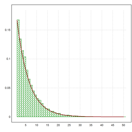
Let us show the distribution of the data and add the expected distribution
![]()
>k=1:50; ...
 plot2d(k,getmultiplicities(k,r)/length(r),>bar,style="/"); ...
 k=1:50; plot2d(k,(5/6)^(k-1)/6,color=red,thickness=2,>add):

Of course, the exact answer is 6.
One direct way to show this is to compute the expected value of n, where the event n occurs, if there is a 6 at the n-th throw, and no 6 before that.
With the default methods, Maxima cannot evaluate the following sum, which would be our result.
>su &= sum(n*(5/6)^(n-1)*1/6,n,1,inf)|simpsum
                            inf
                            ====     n - 1
                            \     n 5
                             >    --------
                            /         n
                            ====     6
                            n = 1
There is the package simplify_sum, which can handle many sums.
>&load(simplify_sum); &simplify_sum(su)
6
Alternatively, we can use the following trick.
>&assume(abs(x)<1); &sum(x^n,n,1,inf)|simpsum
                                  x
                                -----
                                1 - x
Then we have
>&diff(x^n,x)
                                  n - 1
                               n x
Thus, we get our result in the following way.
>&diffat(x/(1-x),x=5/6)*1/6
6
A simpler reasoning is the following: If we simulate dice throws, we get n/6 out of n dice throws. By simple arithmetic, the mean distance between two throws of a 6 is 6.
If we know that the expected time is finite, there is another reasoning. If N is the average waiting time, then N must satisfy
![]()
The reason is: With probability 1/6 we have a 6 in one throw, and with probability 5/6 we have to wait another N throws on average. From this, we get N=6.
>&solve(N=1/6+5/6*(N+1))
[N = 6]
Our next problem is to determine the average waiting time, until we get all numbers on a dice at least once.
We setup a Monte Carlo simulation of one try. To determine when we have all dices for the first time, we take the maximum of the indices of the first time appearance of each number.
>function tryone (n:index=100) ...
 k=intrandom(1,n,6);
 r=0;
 loop 1 to 6
   r=max(r,min(nonzeros(k==#)));
 end;
 return r
 endfunction
>tryone
11
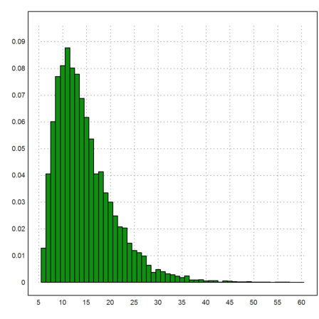
Now we do that 10000 times, and denote the results in a vector.
>m=10000; s=zeros(1,m); ...
 loop 1 to m; s[#]=tryone(); end; ...
 k=6:60; plot2d(k-0.5,getmultiplicities(k,s)/m,>bar):

The following is the mean.
>mean(s)
14.5576
What is the exact answer?
To answer this, assume you have already 4 different dice throws. How long will you have to wait for the fifth? Using the same reasoning as above, you get a waiting time of 1/p, where p=2/6 is the chance to throw a new number, one of the two remaining.
So all we have to do is add these expectation times starting with p=5/6. Note we have to add 1 for our first dice throw.
>1+sum(6/(1:5))
14.7
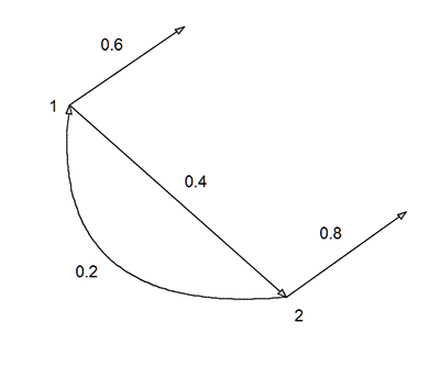
We start with a special problem: Two players throw a Basketball in turn. The first one hits with p1=0.6, and the second one with p2=0.8. How long does the game take on average?
The probabilities of the transitions between the two states can be seen in the following graph.

Now, if N1 is the average time a game takes if the first player starts, and N2 is the average time a game takes if the second player starts, we get the following equations.
![]()
![]()
>&solve([N1=0.6+0.4*(N2+1),N2=0.8+0.2*(N1+1)]), &float(%[1])
                                30       35
                         [[N2 = --, N1 = --]]
                                23       23


           [N2 = 1.304347826086957, N1 = 1.521739130434783]
For the probabilities to win we have a similar set of equations.
![]()
![]()
The reason is: The first player wins immediately in 0.6 of all cases and if not, he has another chance in 0.4*0.2 of all cases. The second player wins immediately only if the first player looses and he wins.
>&solve([w1=0.6+0.4*0.2*w1,w2=0.4*0.8+0.2*0.4*w2])
                                8        15
                         [[w2 = --, w1 = --]]
                                23       23
Let us try to simulate this. This time we use an ordinary loop.
>function esimulate (n) ...
 Sum=0;
 loop 1 to n
   N1=1; // length of game when player 1 starts
   repeat
     until random<0.6;
     N1=N1+1;
     until random<0.8;
     N1=N1+1;
   end
   Sum=N1+Sum;
 end;
 return Sum/n;
 endfunction
On my computer (1.6GHz dual core), I can simulate 1 million runs in about 10 seconds.
>tic; esimulate(1000000), toc;
1.522633
Used 3.022 seconds
With the following C file, we can hope to be much faster.
>cd(eulerhome()); function tinyc simulate(n) ...
 ARG_INT(n);
 CHECK(n>1,"Need an integer >1");
 int i,l;
 double lsum=0;
 for (i=0; i<n; i++)
 {
   l=1;
   while (1)
   {
     if (rand()%100<60) break;
     l+=1;
     if (rand()%100<80) break;
     l+=1;
   }
   lsum+=l;
 }
 new_real(lsum/n);
 endfunction
And simulate 200 million runs. On my computer, this takes about 10 seconds. So the C code is 200 times faster. Euler, like Matlab, is not a good choice for programs with loops.
>tic; simulate(200000000), toc;
1.520613615
Used 4.735 seconds
We can represent the graph with transition probabilities in a matrix P, where P[i,j] is the probability of a transition from i to j. The probabilities to exit from a node are not in the matrix, but can, of course, be implicitly computed.
Following the reasoning above, we get a vector for the vector N, where N[i] is the average waiting time for an exit off the graph assuming we start at node i,
![]()
where 1 is the vector with all ones. Note that 1-P.1 is the vector of probabilities to exit from each node. We get the system
![]()
>P=[0,0.4;0.2,0]
            0           0.4
          0.2             0
This is the matrix of our example of Basketball. We get the same result.
>E=[1;1]; (id(2)-P)\E
      1.52174
      1.30435
We can do the dice example in the same way. Our states are to need 1,2,3,4,5 different dice throws. From the state of k different dices, we remain in this state with probability k/6, and change to state with k+1 different dices with probability (6-k)/6.
>P=diag(5,5,1,(5:-1:1)/6)+diag(5,5,0,(1:5)/6); fracprint(P)
      1/6       5/6         0         0         0
        0       1/3       2/3         0         0
        0         0       1/2       1/2         0
        0         0         0       2/3       1/3
        0         0         0         0       5/6
We find that we need 13.7 throws to exit from state 5 on average. if we start in state 1. Adding the first throw, we get the same result 14.7 as above.
>(id(5)-P)\ones(5,1)
         13.7
         12.5
           11
            9
            6
This is question, where the quick answer "36" is wrong. We have just two states: Last throw wasn't a 6 or it was. From the second state, we exit with probability 1/6.
>P=[5/6,1/6;5/6,0]; fraction P
      5/6       1/6
      5/6         0
Starting in the first state, we have to pass through the second state and then exit there to get two successive 6. This will take 42 throws on average.
>(id(2)-P)\ones(2,1)
           42
           36
Let us simulate that in simple function.
>function tryone () ...
 last = intrandom(6);
 N=1;
 repeat
    dice = intrandom(6);
    N = N+1;
    until last==6 and dice==6;
    last = dice;
 end;
 return N;
 endfunction
Now compute the average over 10000 runs.
>Sum=0; M=10000; loop 1 to M; Sum = Sum+tryone; end; Sum/M,
42.6708
For the matrix language, we could take another approach. We generate 10 Million dice throws.
>m=10000000; v=intrandom(1,m,6);
Now we extract the indices, where v[i]=6 and v[i+1]=6.
>i=nonzeros(v[1:m-1]==6 && v[2:m]==6);
Then we compute the distances between these indices. As expected the mean value of the distances is 36.
>d=differences(i); mean(d)
35.9470602191
But we did not count correctly. After two 6, we have to skip both of them and start counting.
We need an EMT function which marks pairs of 6, but skips after each marked pair for the next mark. This is a tedious and slow function in a loop in EMT. We better do that into a compiled function.
>cd(eulerhome()); function tinyc markpairs (v,number) ...
 ARG_DOUBLE_MATRIX(v,r,c);
 ARG_DOUBLE(number);
 RES_DOUBLE_MATRIX(m,1,c);
 int i;
 for (i=0; i<c; i++) m[i]=0;
 for (i=0; i<c-1; i++)
 {
    if (v[i]==number && v[i+1]==number)
    {
        m[i]=1; i++;
    }
 }
 endfunction
>mean(differences(nonzeros(markpairs(v,6))))
41.9652398338
We can ask, how often we visit the first node in our Basketball example. Again, we can easily simulate this.
In the following function, we start at node 1 and count the visits to nodes 1 or 2 in a vector.
>function vsimulate (n) ...
 w=zeros(1,2);
 loop 1 to n
   repeat
     w[1]=w[1]+1;
     until random<0.6;
     w[2]=w[2]+1;
     until random<0.8;
   end
 end;
 return w/n;
 endfunction
>w=vsimulate(1000000)
[1.08692, 0.434745]
For w[1], this is equivalent a problem with one node, where the probability to revisit the node is 1-0.4*0.2. So the expected waiting time for an exit is simply the following.
>1/(1-0.4*0.2)
1.08695652174
We can view that in a different way. If w[i] is the probability to enter the graph at node i, then P'.w is the probability to be at the nodes after one transition. We get for the expected number of times we are at each node
![]()
Or
![]()
>P=[0,0.4;0.2,0]; (id(2)-P')\[1;0]
      1.08696
     0.434783
This agrees with our simulation.
Let us simulate a general transition matrix to find out the expected number of visits and the mean exit time. We start at node kstart, and use find() for the transition from node p. find() finds a number in a sorted vector. We can use the cumulated probabilities in each line of P.
>function Psimulate (P,m,kstart) ...
 S=cumsum(P);
 n=cols(P);
 w=zeros(1,n);
 lsum=0;
 loop 1 to m;
   p=kstart;
   repeat;
     lsum=lsum+1;
     w[p]=w[p]+1;
     i=find(S[p],random());
     while i<n;
     p=i+1;
   end;
 end;
 return {lsum/m,w/m};
 endfunction
>P=random(5,5); P=P/sum(P)*random(5,1);
>{lmean,w}=Psimulate(P,100000,1); lmean
1.31538
This mean agrees with our general result.
>(id(5)-P)\ones(5,1); %[1]
1.31618821103
The simulated number of visits is the following.
>w
[1.07005, 0.059, 0.02984, 0.03736, 0.11913]
Again, this will agree with our general result.
>(id(5)-P')\[1;0;0;0;0]
      1.07165
    0.0587641
    0.0301114
      0.03752
     0.118147
We might often want to know the expected number of exits from each node. In our Basketball example, this would be the expected number of wins.
Of course, a similar code as above works for a simulation.
>function WinSimulate (P,m,kstart) ...
 S=cumsum(P);
 n=cols(P);
 w=zeros(1,n);
 loop 1 to m;
   p=kstart;
   repeat;
     i=find(S[p],random());
     if i>=n then w[p]=w[p]+1; break; endif;
     p=i+1;
   end;
 end;
 return w/m;
 endfunction
>P=[0,0.4;0.2,0]; WinSimulate(P,10000,1)
[0.648, 0.352]
As we know, the expected values are the following.
>[15,8]/23
[0.652174, 0.347826]
There is a simple way to find this. Each time we visit node 1, we have an exit probability of 0.6. The same for node 2 with exit probability of 0.8. So we can just compute our expected number of visits, and multiply with the exit probabilities.
>(id(2)-P')\[1;0]*[0.6;0.8]
     0.652174
     0.347826
Let us try a larger example.
>P=random(5,5); P=P/sum(P)*random(5,1);
>WinSimulate(P,100000,1)
[0.30279, 0.0989, 0.19697, 0.3658, 0.03554]
>(id(5)-P')\[1;0;0;0;0]*(1-sum(P))
     0.300519
    0.0987227
     0.199436
     0.365919
    0.0354039